How to Predict A Popular Article with Machine Learning (Part 2)

This is part 2 of applying machine learning to practical business problems. Part 1 here. We are working on trying to build a model to predict if an article on Lifehack will become popular or not.

Overview

In Part 1 we have gone through the whole data preparation process, which involves data collection, data preprocessing and data transformation. We will now build a priliminary model with the training and testing data.

Class Imbalance Problem

Remember we partitioned our training and testing data as follows, visualized:

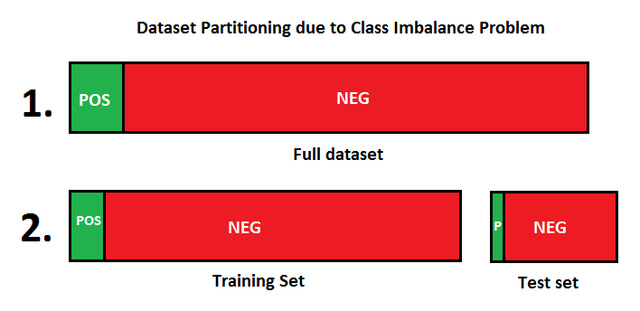
Due to having a lot more negative data than positive data in the training set, our trained model performance will be very poor, despite we supplied a lot of training data. To resolve this, one way is undersampling, which we will throw away negative data. Counter-intuitively, this actually helps. This is called the Class Imbalance Problem.

Dataset Preparation Revisited

Because of the class imbalance problem, we want to keep the training set with 1:1 ratio of positive to negative data, visualized:

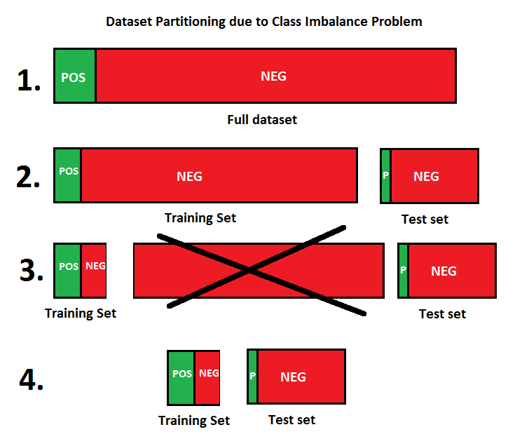
In step 3 of the figure, we throw away a large number of negative examples in the training set. In step 4, we see that the training set is now much smaller with equal number of positive and negative data. This will be the training set we will use. There is no change to the testing set.

How to Choose a Machine Learning Algorithm

There are a lot of models to pick from, such as Random Forest, Support Vector Machines, Linear Regression, Logistic Regression, Gradient Boosted Models, etc… how do we start?

Try something fast, and simple. Preferably with few parameters. So you have a quick turnaround to get a feeling of the dataset and problem at hand. Linear models are a good start. SVMs are not, because you would have to tune the C and gamma parameters, and they are in generally very slow compared to linear models.

In this case, we will pick the Ridge Classifier of Scikit-Learn as our first attempt. It is a linear model, and is relatively first. In practice, it also performs quite well.

How to Get Data Into the Model

The Ridge expects an input matrix of shape {number of examples, number of features} and a vector, the target class. Yet, our training data is a list of text articles. What do we do?

We can use TfidfVectorizer to construct a TF-IDF matrix for our training data. Basically, it converts the text article to a matrix representation of the words suitable for our machine learning algorithm to take in.

After this transformation, we now have an input matrix of shape {number of examples, number of features}.

Connecting the Above Altogether

We refined our training set, converted the data to a matrix for training. We are now ready for a first run! The model in Python Scikit Learn looks like this (with parameters omitted for clarity):

model = Pipeline([
    ('fe1', TfidfVectorizer()),
    ('clf', RidgeClassifier(alpha = 1.0)),
])

The Pipeline is just a construct in Scikit Learn to streamline the data transformation and training. We can now use the model to start training on the training data.

Picking a Score Function

We want to know how good we perform. You may be attempted to use accuracy score, but no. If there are 10000 articles with only 5 positive examples, classifying all articles as negatives will give you an impressive 99.x% accuracy. Apparently, this is a bad model.

Instead, we will use the Receiver Operating Characteristic Area Under Curve (ROC_AUC) score function, which is much more informative by considering true positive rates and false positive rates. A perfect model will have 1.0 score, and a random model will have 0.5 score. A model with less than 0.5 score is useless.

If we use the example above, suppose we classify all examples as negative and get 9995 classifications right, the ROC_AUC will be just 0.5, which means it is completely random.

Results from First Attempt

This model we use yielded and ROC_AUC score of about 0.50~60 on the testing set.

What? Just a bit better than random! How come?

If you have tried toy datasets, it is painfully easy to get a 95% accuracy. However, we are dealing with real data here. It needs optimization effort.

As a best practice, it is a good idea to get something work first, we will then fine tune from there. In fact, machine learning isn’t a one-shot thing. You improve it iteratively, just like you would do in software engineering.

In part 3, I will talk about how to improve this poor preliminary model and how to make sure it performs well on testing data.