Explain to Me : What is the Kernel Trick?
The Kernel Trick is a technique in machine learning to avoid some intensive computation in some algorithms, which makes some computation goes from infeasible to feasible.
So how is it applied?
Concretely, when you see the pattern of xiT xj ( the dot product of xi transpose and xj , where x is an observation ): xiT xj can be replaced by K(xi xj). Here, K is a kernel, which has many implementations: linear, polynomial, RBF, etc.
Give me an example.
The most well-known case would be the Support Vector Machines. The problem state of SVM is a constrained optimization problem as follows:
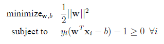
To solve the above efficiently, usually the problem is modeled by as a Lagrange primal problem statement[1] (above) but solved by the dual version of problem statement, which becomes the following:
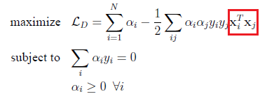
Notice the red I boxed above, that is a very computationally intensive operation. Suppose x is a (10000 x 1) vector, the dot product would introduce 10000 * 10000 = 100000000 multiplications. Suppose you use a linear kernel K(xi, xj) to replace the above red boxed part, there will be only ~10000 multiplications.
It means it is ~10000 times faster.
Conclusion
Machine learning, in practice, will always try to model problems into above or other ways such that the problem can be solved much more efficiently. The Kernel Trick is one of the most important one. The above is an extremely simplified version of what happened only, interested readers should dive deeper into related literature.
[1] – The primal and dual (together called the duality) are the two sides of the problem, which solving the dual problem statement gives the optimal solution to the primal problem statement (under some constraints). This is grossly simplified.
Ref: