Differences between the L1-norm and the L2-norm (Least Absolute Deviations and Least Squares)
[edit: 12/18/2013 Please check this updated post for the rewritten version on this topic. I’m keeping this only for archival purposes. Thanks. ]
[edit: 12/03/2013 As Miroslaw pointed out, there is some confusion here, which I’ll address later in another post. Thanks.]
While practicing machine learning, you may have come upon a choice of deciding whether to use the L1-norm or the L2-norm for regularization, or as a loss function, etc.
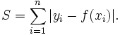
L1-norm is also known as least absolute deviations (LAD), least absolute errors (LAE). It is basically minimizing the sum of the absolute differences (S) between the target value (Yi) and the estimated values (f(xi)):
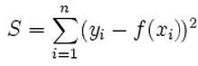
L2-norm is also known as least squares. It is basically minimizing the sum of the square of the differences (S) between the target value (Yi) and the estimated values (f(xi):
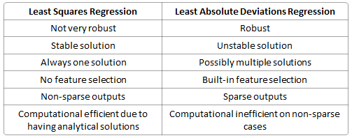
The differences of L1-norm and L2-norm can be promptly summarized as follows:
Robustness, per wikipedia, is explained as:
The method of least absolute deviations finds applications in many areas, due to its robustness compared to the least squares method. Least absolute deviations is robust in that it is resistant to outliers in the data. This may be helpful in studies where outliers may be safely and effectively ignored. If it is important to pay attention to any and all outliers, the method of least squares is a better choice.
Intuitively speaking, since a L2-norm squares the error (increasing by a lot if error > 1), the model will see a much larger error ( e vs e2 ) than the L1-norm, so the model is much more sensitive to this example, and adjusts the model to minimize this error. If this example is an outlier, the model will be adjusted to minimize this single outlier case, at the expense of many other common examples, since the errors of these common examples are small compared to that single outlier case.
Stability, per wikipedia, is explained as:
The instability property of the method of least absolute deviations means that, for a small horizontal adjustment of a datum, the regression line may jump a large amount. The method has continuous solutions for some data configurations; however, by moving a datum a small amount, one could “jump past” a configuration which has multiple solutions that span a region. After passing this region of solutions, the least absolute deviations line has a slope that may differ greatly from that of the previous line. In contrast, the least squares solutions is stable in that, for any small adjustment of a data point, the regression line will always move only slightly; that is, the regression parameters are continuous functions of the data.
This is best explained with a picture below (mspaint made, sorry for the low quality):
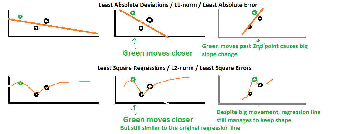
The top represents L1-norm and the bottom represents L2-norm. The first column represents how a regression line fits these three points using L1-norm and L2-norm respectively.
Suppose we move the green point horizontally slightly towards the right, the L2-norm still maintains the shape of the original regression line but makes a much steeper parabolic curve. However in the L1-norm case, the slope of the regression line is now much more steeper affecting every other predictions even well-beyond the rightmost point. As such, all future predictions are affected much more seriously than the L2-norm results.
Suppose we move the green point even more horizontally further to the right past the first black point (third column), the L2-norm now also changes a bit but not as much as the L1-norm, which the slope has completed turned in direction. This change of slope will definitely invalidate all previous results.
By just a small perturbation of the data points, the regression line changes by a lot. This is what instability of the L1-norm (versus the stability of the L2-norm) means here.
Solution uniqueness is a simpler case but requires a bit of imagination. First, this picture below:
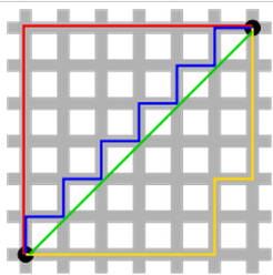
The green line (L2-norm) is the unique shortest path, while the red, blue, yellow (L1-norm) are all same length (=12) for the same route. Generalizing this to n-dimensions. This is why L2-norm has unique solutions while L1-norm does not.
Built-in feature selection is frequently mentioned as a useful property of the L1-norm, which the L2-norm does not. This is actually a result of the L1-norm, which tends to produces sparse coefficients (explained below). Suppose the model have 100 coefficients but only 10 of them have non-zero coefficients, this is effectively saying that “the other 90 predictors are useless in predicting the target values”. L2-norm produces non-sparse coefficients, so does not have this property.
Sparsity refers to that only very few entries in a matrix (or vector) is non-zero. L1-norm has the property of producing many coefficients with zero values or very small values with few large coefficients.
Computational efficiency. L1-norm does not have an analytical solution, but L2-norm does. This allows the L2-norm solutions to be calculated computationally efficiently. However, L1-norm solutions does have the sparsity properties which allows it to be used along with sparse algorithms, which makes the calculation more computationally efficient.
References:
[[edit: 12/18/2013 Please check this updated post for the rewritten version on this topic. I’m keeping this only for archival purposes. Thanks. ]
[edit: 12/03/2013 As Miroslaw pointed out, there is some confusion here, which I’ll address later in another post. Thanks.]