Meanshift Algorithm for the Rest of Us (Python)
What is Meanshift?
Meanshift is a clustering algorithm that assigns the datapoints to the clusters iteratively by shifting points towards the mode. The mode can be understood as the highest density of datapoints (in the region, in the context of the Meanshift). As such, it is also known as the mode-seeking algorithm. Meanshift algorithm has applications in the field of image processing and computer vision.
Given a set of datapoints, the algorithm iteratively assign each datapoint towards the closest cluster centroid. The direction to the closest cluster centroid is determined by where most of the points nearby are at. So each iteration each data point will move closer to where the most points are at, which is or will lead to the cluster center. When the algorithm stops, each point is assigned to a cluster.
Unlike the popular K-Means algorithm, meanshift does not require specifying the number of clusters in advance. The number of clusters is determined by the algorithm with respect to the data.
I wrote this article in case I forgot what Meanshift is. Hopefully I won’t. =]
The Meanshift code is available as a notebook on Github.
Meanshift by Example
Here is a diagram that shows what happens step-by-step in Meanshift.
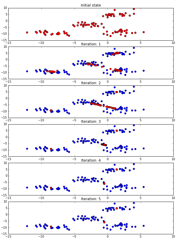
The blue datapoints are the initial datapoints and red are the positions of those datapoints at each iteration. Description for each step:
Iteration:
- Initial state. The red and blue datapoints overlap completely in the first iteration before the Meanshift algorithm starts.
- End of iteration 1. All the red datapoints move closer to clusters. Looks like there will be 4 clusters.
- End of iteration 2. The clusters of upper right and lower left seems to have reached convergence just using two iterations. The center and lower right clusters looks like they are merging, since the two centroids are very close.
- End of iteration 3. No change in the upper right and lower left centroids. The other two centroids’ have pulled each other together as the datapoints affect each clusters. This is a signature of Meanshift, the number of clusters are not pre-determined.
- End of iteration 4. All the clusters should have converged.
- End of iteration 5. All the clusters indeed have no movement. The algorithm stops here since no change is detected for all red datapoints.
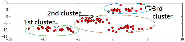
Meanshift found 3 clusters here, which I circled out above. The original data is actually generated from 4 clusters of data, but Meanshift thinks 3 can represent the set of data better, and it’s not too bad. I used Scikit-Learn’s datasets make_blobs:
make_blobs(100, 2, centers=4, cluster_std=1.3)
Now we have a big picture of how Meanshift works overall. Let’s look into what is a single datapoint is doing, and generalize that to all points.
Just A Single Datapoint
Below we run a single datapoint through Meanshift iteratively on a new set of datapoints. The single datapoint is pointed to by the black arrow.
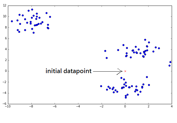
The closest cluster of points could be south or north of the initial datapoint. One can tell by inspecting the data that running the Meanshift algorithm should bring the datapoint closer either to the datapoints to the south or north.
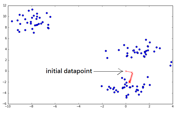
The red path shows that the point moves closer to the southern cluster center after each iteration. One may notice the movement decreases gradually after each iteration, and that is because the datapoint is closer to the centroid so the shift is less drastic. After 10 iterations, the point is really close to the centroid. The meanshift does this for all datapoints for K iterations. In most cases, 5 iterations should suffice for convergence. From this we can tell the algorithm’s runtime complexity is O(KN2), where N is the number of datapoints and K is the number of iterations of Meanshift.
Note that this implementation to demonstrate a single point moving is slightly different to where all the datapoints are moving, but the idea is basically the same. For the curious, if all the datapoints move, it will affect each neighbouring datapoints more drastically. The result is that the algorithm converges faster: ~3 iterations above versus ~10 iterations in this version.
The Meanshift Algorithm
I will have to touch lightly on the mathematics for this part. I hate math so I will try my best to explain in terms for non-math people.
You will need a few things before you start to run Meanshift on a set of datapoints X:
- A function N(x) to determine what are the neighbours of a point x ∈ X. The neighbouring points are the points within a certain distance. The distance metric is usually Euclidean Distance.
- A kernel K(d) to use in Meanshift. K is usually a Gaussian Kernel, and d is the distance between two datapoints.
Now, with the above, this is the Meanshift algorithm for a set of datapoints X:
- For each datapoint x ∈ X, find the neighbouring points N(x) of x.
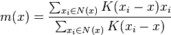
- For each datapoint x ∈ X, calculate the mean shift m(x) from this equation:
- For each datapoint x ∈ X, update x ← m(x).
- Repeat 1. for n_iteations or until the points are almost not moving or not moving.
The most important piece is calculating the mean shift m(x). The formula in step 2. looks daunting but let’s break it down. Notice the red red encircled parts are essentially the same:
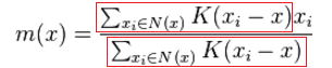
Let’s replace that with Wi, so the formula becomes this:
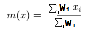
Look at the general formula for weighted average in Wikipedia gives us this:
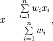
Which is just the same thing! Essentially, the meanshift is just calculating the weighted average of the affected points w.r.t. to x. From this perspective, the formula is less mystifying, right?
To summarize: The algorithm finds a set of nearby points that affect a datapoint, then shift it towards where most of the points are, and the closest points have more influence than the further points. Repeat this for all datapoints until nothing changes.
Code
Define the kernel, euclidean distance, neighbourhood functions we need first:
def euclid_distance(x, xi):
    return np.sqrt(np.sum((x - xi)**2))

def neighbourhood_points(X, x_centroid, distance = 5):
    eligible_X = []
    for x in X:
        distance_between = euclid_distance(x, x_centroid)
        # print('Evaluating: [%s vs %s] yield dist=%.2f' % (x, x_centroid, distance_between))
        if distance_between <= distance:
            eligible_X.append(x)
    return eligible_X

def gaussian_kernel(distance, bandwidth):
    val = (1/(bandwidth*math.sqrt(2*math.pi))) * np.exp(-0.5*((distance / bandwidth))**2)
    return val
Next, we will implement Meanshift by translating the algorithm as described above.
X = np.copy(original_X)

past_X = []
n_iterations = 5
for it in range(n_iterations):
    for i, x in enumerate(X):
        ### Step 1. For each datapoint x ∈ X, find the neighbouring points N(x) of x.
        neighbours = neighbourhood_points(X, x, look_distance)

        ### Step 2. For each datapoint x ∈ X, calculate the mean shift m(x).
        numerator = 0
        denominator = 0
        for neighbour in neighbours:
            distance = euclid_distance(neighbour, x)
            weight = gaussian_kernel(distance, kernel_bandwidth)
            numerator += (weight * neighbour)
            denominator += weight

        new_x = numerator / denominator

        ### Step 3. For each datapoint x ∈ X, update x ← m(x).
        X[i] = new_x

    past_X.append(np.copy(X))
This code is a naive implementation of Meanshift algorithm. There are a lot of optimizations that can be done to improve this code’s speed. For instance, 1) Vectorize the implementation above, 2) Use a Ball Tree to calculate the neighbourhood points much more efficiently, etc.
The code is available on Github.
K-Means VS Meanshift
Meanshift looks very similar to K-Means, they both move the point closer to the cluster centroids. One may wonder: How is this different from K-Means? K-Means is faster in terms of runtime complexity!
The key difference is that Meanshift does not require the user to specify the number of clusters. In some cases, it is not straightforward to guess the right number of clusters to use. In K-Means, the output may end up having too few clusters or too many clusters to be useful. At the cost of larger time complexity, Meanshift determines the number of clusters suitable to the dataset provided.
Another commonly cited difference is that K-Means can only learn circle or ellipsoidal clusters. However, this is not true. The reason that Meanshift can learn arbitrary shapes is because the features are mapped to another higher dimensional feature space through the kernel. The arbitrary shapes are due to the algorithm finding circle or ellipsoidal clusters in higher dimensional feature space. When the features are mapped back to 1D/2D/3D, the resulting clusters look like strange shapes. This is also the trick as used in Support Vector Machines.
A traditional K-means does not use kernels, but Kernel K-means is available. Kernel K-Means is useful if 1) the number of clusters is known or can be reasonably estimated, and 2) dataset needs learning non-ellipsoidal cluster shapes. So, you can enjoy the better runtime complexity of K-Means and learn arbitrary clusters if you can determine the number of clusters to use.
Applications
Image Processing
Meanshift is used as an image segmentation algorithm. Here is what Meanshift can do for us:
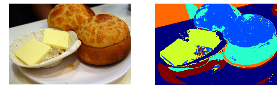
The idea is that similar colors are grouped to use the same color. Using a library called Scikit-Learn, this can be done very easily. The gist of the code is this:
ms = MeanShift(bandwidth=bandwidth, bin_seeding=True)
ms.fit(X)
You can find an end-to-end working code on Github in this notebook.
EFavDB has an excellent article on this topic which I highly recommend.
Computer Vision
Meanshift is used as an object tracking algorithm. The idea is that you need to identify the target to track, and build a color histogram of this target, and then keep on sliding the tracking window to the closest match (the cluster center) to keep up with the target to track. Here is an animated gif from OpenCV that illustrates this:
You can find more details and OpenCV code demonstration here.
Summary
By now we should understand that Meanshift is a simple and versatile algorithm that finds applications in general data clustering, image processing and object tracking. It has similarities with K-Means but there are differences. Meanshift is essentially iterations of weighted average of the datapoints. Hopefully this article unravels some of the technical details that bothers you.
References
- https://en.wikipedia.org/wiki/Mean_shift
- https://spin.atomicobject.com/2015/05/26/mean-shift-clustering/
- http://stackoverflow.com/questions/4831813/image-segmentation-using-mean-shift-explained
- http://homepages.inf.ed.ac.uk/rbf/CVonline/LOCAL_COPIES/TUZEL1/MeanShift.pdf
- http://scikit-learn.org/stable/modules/clustering.html
- https://saravananthirumuruganathan.wordpress.com/2010/04/01/introduction-to-mean-shift-algorithm/
- The estimation of the gradient of a density function, with applications in pattern recognition